
Congratulations! You've landed an interview I understand, and now it's time to prepare for it!
One of the most important guides at your disposal is this interview guide. think of it as your roadmap to success, guiding you through the twists and turns of the interview process. Here's how to decode and utilize this essential document effectively.

Start by carefully reading through this interview guide from start to end. Pay attention to any instructions, formatting, or specific questions provided.
Spend time on each topic, take notes, strive for understanding, and, most importantly, attempt to model these complex problems using either Excel or Python.
While this interview guide provides a detailed framework, be prepared to adapt and think on your feet. Interviewers may ask unexpected or follow-up questions to test deeper into certain areas.
After the interview, reflect on your performance and seek feedback from trusted sources, such as mentors, career advisors, or interview coaches. Again, take notes of areas of improvement and incorporate them into your preparation for future interviews.
Modeling Term-Structure of Interest Rates
What are the underlying factors driving change in interest rates:
Interest rates are influenced by a multitude of factors, both macroeconomic and market-specific. Some of the primary factors affecting interest rates include:
Monetary Policy: Central banks adjust short-term interest rates to manage inflation, unemployment, and economic growth. Changes in central bank policy rates, such as the Federal Reserve's federal funds rate or the European Central Bank's refinancing rate, can have a significant impact on interest rates across the yield curve.
Inflation Expectations: Expectations about future inflation rates influence nominal interest rates. Higher expected inflation tends to lead to higher nominal interest rates to compensate investors for the erosion of purchasing power.
Economic Indicators: Economic data releases, such as GDP growth, employment reports, and consumer price indices, provide insights into the health of the economy and can affect interest rate expectations. Strong economic data may lead investors to anticipate higher future interest rates, while weak data may lead to expectations of lower rates.
Global Economic and Geopolitical Events: Developments in global financial markets, geopolitical tensions, and other macroeconomic events can impact investor sentiment and influence interest rates.
Understanding these factors and their interplay/correlation is crucial for accurately assessing interest rate risk and its potential impact on fixed-income portfolios.
How would you construct an interest rate curve from market data?
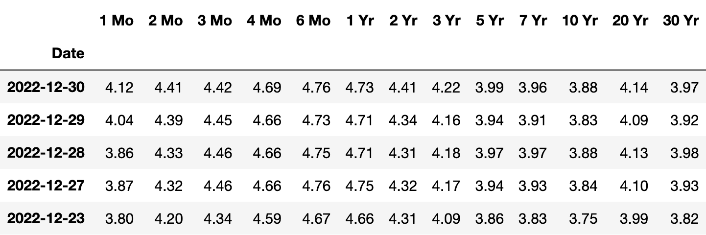
To construct a yield curve from market data, the first step is to gather spot rate data on bonds of different maturities. Then we can plot the spot rates against the time to maturity for each bond. By doing this, a yield curve can be created that can be used to estimate the yield for bonds with maturities. The yield curve can be smoothed using a statistical technique like spline interpolation to remove any noise or irregularities in the data.
What are the implications of different shapes of yield curves?
A yield curve is a graphical representation of the interest rates for a range of maturities of bonds or other fixed-income securities. It shows the relationship between the interest rate (or cost of borrowing) and the time to maturity of the debt.
Different shapes of yield curves can have different implications for the economy and financial markets.
Normal Yield Curve: A normal yield curve, also known as a positive or upward-sloping yield curve, occurs when longer-term interest rates are higher than shorter-term interest rates. In other words, as the time to maturity increases, so does the yield or interest rate. This is the most common shape of the yield curve and reflects the expectation of future economic growth. Investors typically demand higher compensation for lending money over a longer period due to increased uncertainty and inflation risks. A normal yield curve is often seen as a sign of a healthy economy and can be associated with a bull market in stocks. For example, from 2003 to 2006, the US yield curve was normal, with the yield on 10-year Treasury bonds higher than the yield on 3-month Treasury bills. During this time, the US stock market experienced strong growth and the economy expanded at a moderate pace.
Inverted Yield Curve: An inverted yield curve, also known as a negative or downward-sloping yield curve, is the opposite of a normal yield curve. It occurs when shorter-term interest rates are higher than longer-term interest rates. In other words, as the time to maturity increases, the yield or interest rate decreases. An inverted yield curve is considered a potential warning sign of an economic downturn or recession. It suggests that investors have a pessimistic view of the future and expect interest rates to decline in the long run due to anticipated central bank actions to stimulate the economy. An inverted yield curve is often seen as a warning sign of an impending economic downturn or recession. For example, in late 2005 and early 2006, the US yield curve became inverted, with the yield on 3-month Treasury bills higher than the yield on 10-year Treasury bonds. This inversion was followed by the 2008 financial crisis and subsequent recession. [One could consider quoting an example of the current market condition to further support the explanation!]
Humped Yield Curve: A humped yield curve, also known as a flat or bell-shaped yield curve, is characterized by a temporary increase in interest rates for intermediate-term maturities, creating a slight "hump" in the curve. It means that the yields for bonds with medium-term maturities are higher than both shorter-term and longer-term maturities. A humped yield curve often reflects a period of uncertainty or mixed market expectations about the future direction of interest rates. It can occur during transitional phases in the economy, such as changing monetary policy or economic conditions. A flat yield curve can signal uncertainty or a lack of confidence in the economy. For example, from 2006 to 2007, the US yield curve was relatively flat, with the yield on 10-year Treasury bonds only slightly higher than the yield on 3-month Treasury bills. During this time, there was growing concern about the housing market and the subprime mortgage crisis, which eventually led to the 2008 financial crisis.
It's important to note that yield curves are not fixed and can change over time based on various factors, including economic conditions, inflation expectations, central bank policies, and market sentiment. The shape of the yield curve provides insights into market expectations and investor sentiment regarding future interest rates and economic conditions.
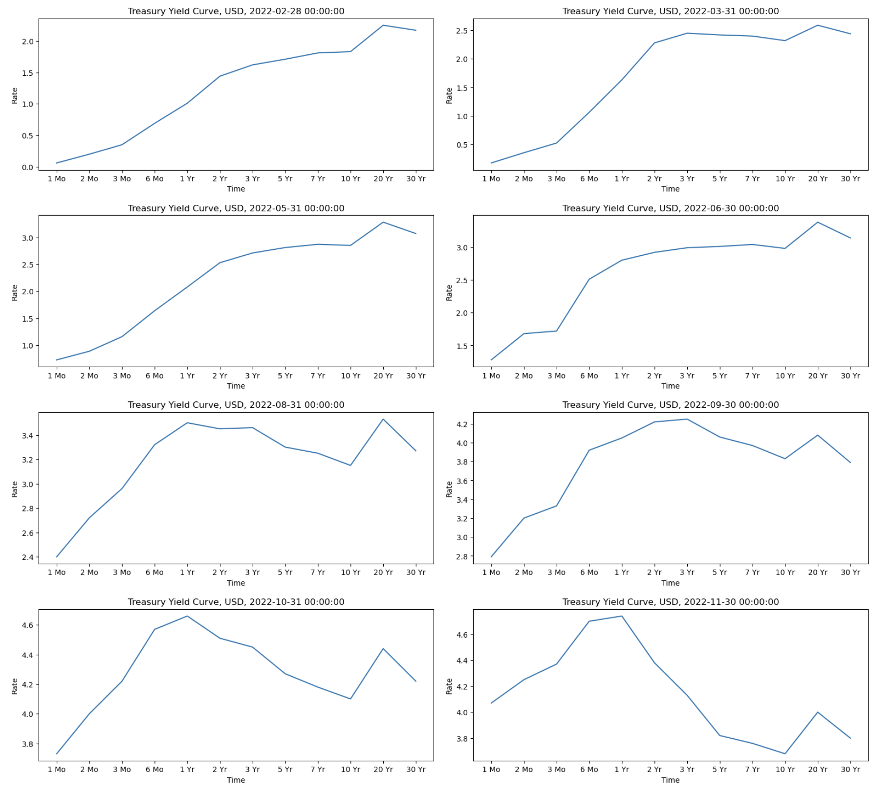
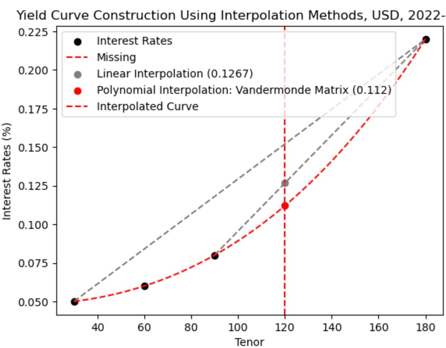
Explain the concept of linear interpolation in the context of constructing an interest rate yield curve.
How does the linear interpolation method help in estimating interest rates for intermediate maturities?
The linear interpolation method is commonly used for constructing the yield curve, especially when there are gaps or missing data points. It involves estimating the interest rates for intermediate maturities based on the known interest rates at nearby maturities. The process involves:
Gather the available interest rate data points for various maturities. These data points can be obtained from government bond yields or other fixed-income securities. Arrange the data points in ascending order based on the respective maturities.
Identify the desired maturity point that requires an estimated interest rate. Locate the two known data points that bracket the desired maturity. One data point should have a lower maturity than the desired point, and the other should have a higher maturity.
Calculate the weightage for each known data point based on their proximity to the desired maturity. The weightage can be determined by taking the difference between the desired maturity and the two known maturities, divided by the difference between the two known maturities.
Apply linear interpolation using the weightage to estimate the interest rate for the desired maturity. This can be done by multiplying the weightage for the lower maturity data point by its corresponding interest rate, and similarly for the higher maturity data point. Then, sum these two values to obtain the estimated interest rate.
Interest Rate (Interpolated) = Interest Rate (Lower Maturity) + (Weightage * [Interest Rate (Higher Maturity) - Interest Rate (Lower Maturity)])
In this equation, the Interest Rate (Interpolated) represents the estimated interest rate for the desired maturity. Interest Rate (Lower Maturity) and Interest Rate (Higher Maturity) refer to the known interest rates for the maturities that bracket the desired maturity. The Weightage represents the weight assigned to the lower maturity interest rate based on the proximity of the desired maturity to the known maturities.
By applying this equation, the linear interpolation method calculates the estimated interest rate by adding a portion of the difference between the higher and lower maturity interest rates based on the weightage assigned to the lower maturity.
Repeat this process for all desired maturities to construct the complete yield curve.
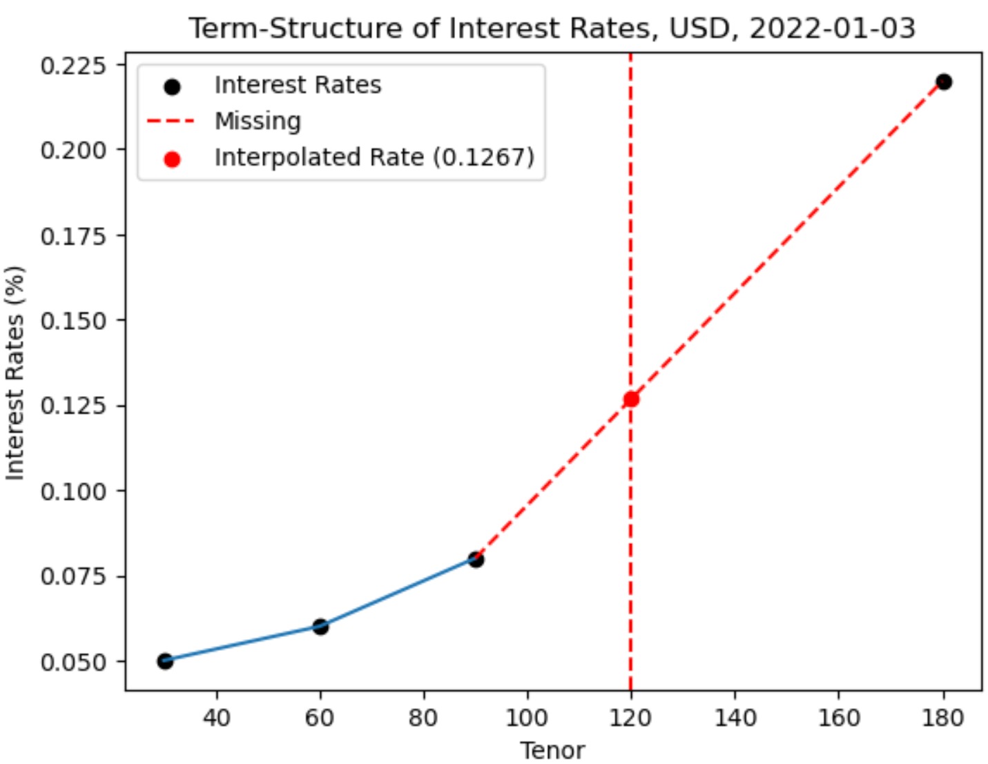
the linear interpolation method assumes a linear relationship between interest rates and maturities. While this method provides a straightforward approach, there are other advanced interpolation techniques available, such as the Vandermonde Matrix, Newton's Divided Difference, Lagrange Interpolation method, Quasi-Cubic Hermite Spline method, Monotone Convex Spline (MC) method, that capture more complex yield curve dynamics.
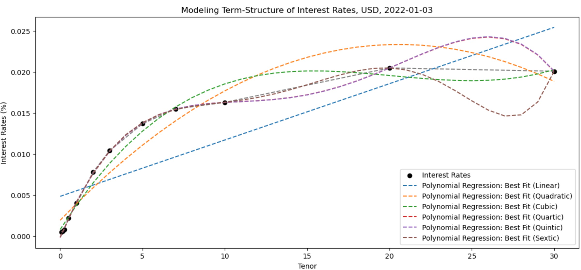
What are the assumptions and limitations associated with Cubic Spline interpolation?
Cubic Spline interpolation is a mathematical technique used to estimate the values of interest rates at missing tenors in yield curve construction.


It constructs a curve that smoothly passes through the given data points and provides estimates for intermediate values. However, there are certain assumptions and limitations associated with it.
It assumes the yield curve is continuous and exhibits smooth movements between data points.
It treats all data points equally and may not effectively handle outliers or extreme values.
It is primarily used for estimating values between known data points and does not provide predictive capabilities beyond the range.
Various factors, such as liquidity factors, supply-demand imbalances, and structural breaks, can introduce complexities and irregularities in the yield curve, difficult to capture.
The quality and distribution of data points used for interpolation can significantly affect the results.
There is a risk of overfitting the data in the case of higher-order polynomials.
It may not have a direct economic or financial interpretation.
to address these limitations and capture the irregularities in the yield curve, additional techniques and advanced models should be applied to enhance the accuracy and reliability of yield curve construction. We don't forget to assess the limitations and adapt the methodologies based on the specific requirements and characteristics of the yield curve construction process.
Why might we choose to use regression models for yield curve construction when we have the option to interpolate? What specific advantages or insights do regression models offer in this context?
Choosing between regression models and interpolation methods in yield curve construction depends on the objectives of the analysis and the characteristics of the available data.
Interpolation is crucial when we have a set of discrete data points and need to estimate interest rates for tenors that fall between those observed points. It is particularly useful for creating a smooth and continuous curve representation. While interpolation excels at local accuracy within the observed range, it may not capture the broader trends or risk factors influencing the entire yield curve.
Regression models are valuable when we aim to understand complex relationships between various factors and interest rates. They allow us to incorporate additional explanatory variables, providing insights into how economic indicators or market conditions influence different segments of the yield curve. Regression models also offer flexibility in capturing overall trends and dynamics. Yield Curve Behavior: The Impact of Multiple Inflection Points
In many cases, a combination of both regression models and interpolation is employed. Regression models can capture the complexity of underlying relationships, while interpolation ensures a seamless and continuous curve for all tenors.
How would you interpret the "y-intercept", "b1", and "b2" coefficients different from "level", "slope", and "curvature" in yield curve analysis?
While there is some similarity in the concepts, it's important to note that the terms "y-intercept," "b1 coefficient," and "b2 coefficient" are more commonly associated with linear regression models rather than the yield curve analysis.
Linear Regression:
Y-Intercept (Intercept): In a linear regression model (y = b0 + b1 * x), the y-intercept (b0) represents the value of the dependent variable (y) when the independent variable (x) is zero. It's the point where the regression line crosses the y-axis.
B1 Coefficient (Slope, first-order/degree): the coefficient b1 represents the slope of the regression line, indicating the change in the dependent variable for a one-unit change in the independent variable.
In a Polynomial Regression:
B2 Coefficient (curvature, second-order/degree): the coefficient b2 represents the curvature or concavity in the quadratic curve of the polynomial regression, indicating the change in the slope of the curve for a one-unit change in the independent variable. A positive b2 indicates an upward-opening parabola, while a negative b2 indicates a downward-opening parabola.
Yield Curve Analysis:
Level: In the context of the yield curve, the level refers to the overall interest rate level across maturities. It's not directly equivalent to the y-intercept but more broadly reflects the prevailing interest rate environment.
Slope: the slope of the yield curve refers to the relationship between short-term and long-term interest rates. It provides insights into the yield spread.
Curvature: the curvature represents the rate at which the yield curve changes direction, indicating the acceleration or deceleration of interest rate changes.
In linear regression, the y-intercept and coefficients are specific parameters of a linear model. In yield curve analysis, the level, slope, and curvature describe different aspects of the yield curve's shape and movement.
What are the key parameters and evaluation metrics used in validating yield curve models, particularly those based on NS and NSS methodologies?
When validating yield curve models, several key parameters and evaluation metrics are commonly used which help to assess the performance of the models and their ability to accurately represent the term structure of interest rates.
Here are some of the key parameters and evaluation metrics used in validating yield curve models:
Model Parameters:
Level (ß0): It represents the long-term interest rate level or the flat yield curve.
Slope (ß1): It reflects the steepness or slope of the yield curve.
Curvature (ß2, ß3, ß4 for NSS model): It captures the curvature or bending of the yield curve. (please note, the NSS model includes additional curvature parameters compared to the NS model.)
Evaluation Metrics:
Mean Absolute Error (MAE): It measures the average absolute difference between observed and predicted interest rates across all maturity points. Lower MAE indicates better model accuracy.
Mean Squared Error (MSE): It calculates the average of the squared differences between observed and predicted interest rates. It penalizes larger errors more heavily than MAE.
Root Mean Squared Error (RMSE): It is the square root of MSE, providing an interpretable measure of error in the same units as the original data.
Median Absolute Error (MedAE): It is the median absolute difference between observed and predicted interest rates, offering a robust measure of central tendency in the error distribution.
Maximum Error (ME): Identifies the maximum absolute difference between observed and predicted interest rates, highlighting potential outliers or extreme errors.
Mean Absolute Percentage Error (MAPE): It calculates the average percentage difference between observed and predicted interest rates, providing insight into relative errors.
Residual Sum of Squares (RSS): It measures the sum of the squared differences between observed and predicted interest rates, evaluating overall model fit.
Total Sum of Squares (TSS): It represents the total variability in the observed interest rates.
Coefficient of Determination (R²): It is also known as the coefficient of determination, R-squared measures the proportion of variability in the observed interest rates that is explained by the model. Higher R² values indicate better model fit.
these parameters and evaluation metrics collectively provide a comprehensive assessment of the accuracy, precision, and overall performance of NS and NSS yield curve models. A successful validation process ensures that the models effectively capture the term structure of interest rates and can be relied upon for various financial applications, including pricing derivatives, risk management, and investment decision-making.
How Principal Component Analysis (PCA) can help in modeling interest rate risk?
Interest rate risk is a significant concern for investors in fixed-income securities, as fluctuations in interest rates can impact the value of their investments. Managing this risk effectively requires understanding the underlying factors driving interest rate movements and their impact on portfolio performance. Principal Component Analysis (PCA) offers a powerful technique for simplifying the complexity of interest rate risk modeling by identifying the most significant drivers of variability in fixed-income portfolios.
PCA is a dimensionality reduction technique commonly used in finance to extract the underlying structure in high-dimensional datasets. It transforms a set of correlated variables into a new set of uncorrelated variables, known as principal components, which capture the maximum variance in the original data. By retaining only the most important components, PCA reduces the dimensionality of the dataset while preserving much of the relevant information.
The reduced set of principal components is used as input variables in risk models for fixed-income portfolios. This simplified representation of interest rate risk factors facilitates more efficient risk analysis and decision-making.
Describe the steps involved in conducting Principal Component Analysis (PCA).
this question assesses the candidate's understanding of the basic procedure of PCA. The candidate should provide a clear and concise explanation of the primary steps involved in PCA without delving into too much technical detail. The response should cover essential aspects such as data preprocessing, calculation of principal components, and interpretation of results, presented straightforwardly.
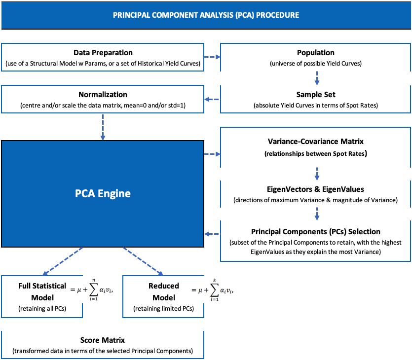
By following these steps, PCA enables dimensionality reduction while retaining the essential information present in the original dataset.
What is a score matrix in Principal Component Analysis (PCA)?
PCA is a dimensionality reduction technique commonly used in data analysis and machine learning. It works by transforming the original variables into a new set of uncorrelated variables called principal components. These principal components are ordered by the amount of variance they explain in the data, with the first principal component capturing the most variance and subsequent components capturing decreasing amounts of variance.
The score matrix in PCA contains the coordinates of the original data points in this new feature space defined by the principal components. Each row of the score matrix corresponds to a data point, and each column corresponds to a principal component. The elements of the score matrix are the projections of the original data points onto the principal components.
What are the benefits of Principal Component Analysis (PCA) in modeling risk factors?
Principal Component Analysis (PCA) offers a practical solution to address the challenges of modeling multiple risk factors in fixed-income portfolios. By applying PCA, investors can:
Dimensionality Reduction: PCA identifies the most significant sources of variability in a dataset and represents them as a smaller set of uncorrelated variables called principal components. This dimensionality reduction simplifies the modeling process and improves computational efficiency.
Common Risk Factors Identification: PCA helps uncover underlying patterns or common factors driving changes in interest rates and fixed-income securities. By focusing on these common factors, investors can better understand the primary drivers of portfolio risk and return.
Interpretability Enhancement: PCA provides a clear and interpretable framework for analyzing complex datasets. By transforming the original variables into principal components, PCA allows investors to identify and interpret the key factors influencing interest rate risk more effectively.
PCA enables investors to gain valuable insights into the underlying structure of fixed-income markets and streamline the modeling process by reducing the number of risk factors to a manageable set of principal components.
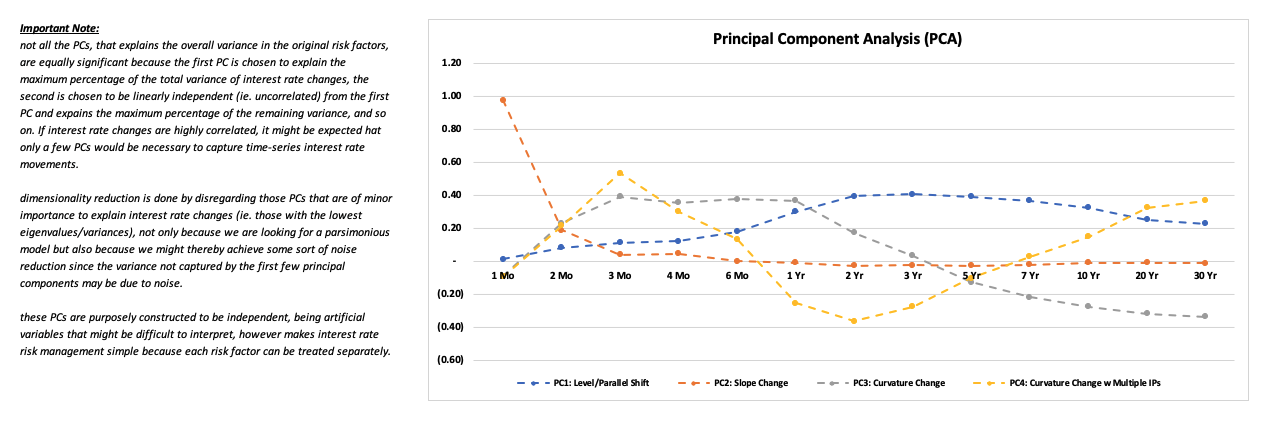
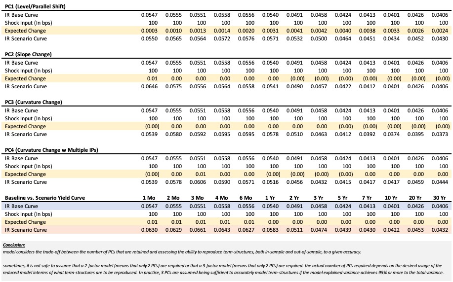
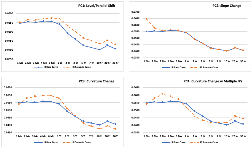
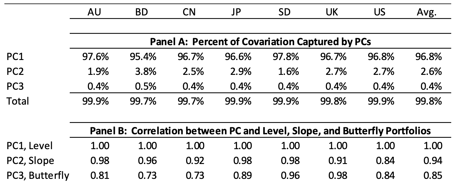
What is the significance of level, slope, and curvature in modeling the term structure of interest rates using Principal Component Analysis (PCA)?
In term structure modeling using PCA, three primary components are typically identified: level, slope, and curvature. these components represent distinct patterns of movement within the term structure and provide valuable insights into interest rate dynamics.
Level Change or Parallel Shift: a level change, which is also known as a parallel shift, refers to a scenario where all interest rates across different maturities move in the same direction by approximately the same amount. » Indicative of a uniform shift in the entire yield curve, often influenced by macroeconomic factors such as changes in monetary policy or economic outlook. » While the magnitude of the shift may vary slightly across different maturities, the overall shape of the yield curve remains relatively unchanged.
Slope Change or Twist: a slope change, which is also known as twist, occurs when short-term interest rates move in one direction while long-term rates move in the opposite direction. » Change in the steepness of the yield curve, resulting in either a flattening or steepening effect. » Typically signals expectations of future economic growth and inflation, while a flattening curve may indicate economic uncertainty or impending recession.
Curvature Change or Turn: a curvature change, which is also referred to as turn, involves movement in the curvature of the yield curve. » Short-term and long-term interest rates move in one direction, while intermediate maturity rates move in the opposite direction. » Reflects changes in market sentiment and expectations, often influenced by factors such as supply and demand dynamics or changes in market liquidity.
Interpreting PCA Components in Term Structure Modeling
In practice, PCA aims to identify a set of principal components that collectively explain a significant portion of the variability in the term structure. three principal components are considered sufficient if they account for 95% or more of the total variance.
by interpreting the factor loading coefficients of each principal component, analysts can determine the contributions of level, slope, and curvature to overall yield curve movements.
» enables better understanding and forecasting of interest rate dynamics,
» assisting in risk management strategies, portfolio optimization, and investment decision-making.
What are the limitations of the Principal Component Analysis (PCA)?
Principal Component Analysis (PCA) is a powerful technique for dimensionality reduction and data visualization. However, it comes with certain limitations:
Linearity Assumption: PCA assumes that the underlying data is linear. If the data exhibits non-linear relationships, PCA might not capture the underlying structure accurately. In such cases, non-linear dimensionality reduction techniques like t-SNE or Kernel PCA may be more appropriate.
Orthogonality Constraint: PCA requires the principal components to be orthogonal to each other. While this aids in simplifying interpretations, it may not always accurately represent the underlying data, especially when the relationships among variables are not strictly orthogonal.
Sensitive to Scale: PCA is sensitive to the scale of the variables. Variables with larger scales can dominate the principal components, leading to biased results. It's crucial to standardize or normalize the data before applying PCA.
Preservation of Variance: PCA retains components that explain the most variance in the data. However, it might not always capture the most relevant information for the specific problem at hand. Important but less variable features might be discarded, leading to a loss of information.
Interpretability: While PCA aids in dimensionality reduction, the resulting principal components might not always have clear interpretations, especially when dealing with a large number of variables. Interpretability can be challenging, particularly when trying to relate the principal components back to the original variables.
Outliers: PCA is sensitive to outliers since it focuses on maximizing variance. Outliers can disproportionately influence the principal components, potentially leading to misrepresentation of the underlying structure.
Despite these limitations, PCA remains a widely used and valuable tool for dimensionality reduction for the term structure of interest rates and volatilities.