Introduction to Jupyter Notebook

Jupyter Notebook is a free, open-source web application for interactive computing. It lets you create computational documents that combine runnable code with text, math equations, charts, and images all in one place. This makes Jupyter very popular for data analysis and automation: you can run code step-by-step, see results immediately, and write explanations or notes alongside.

Notebooks are easy to share (via files, GitHub, email, etc.) and reproduce. Key advantages are that notebooks can contain code, rich text, and visuals together. They support many languages (most commonly Python, R, Julia, and over 40 others), run in your browser, and produce rich outputs (HTML, images, plots, LaTeX, interactive widgets).

Jupyter is therefore ideal for exploratory data work: you can run code interactively (one cell at a time), plot graphs or tables, and write documentation or equations (using Markdown and LaTeX) all in the same document. Its ease-of-use and immediate feedback loop help accelerate analysis, debugging, and sharing results, which is why it’s widely used by data scientists, engineers, and educators.

Figure: Anaconda Navigator showing the Jupyter Notebook tile with a Launch button. Clicking Launch opens the Jupyter Notebook dashboard in your browser

Launching Jupyter Notebook

The most common way to start Jupyter is via the Anaconda Navigator, which comes with the Anaconda Python distribution. Here’s how:

• Open Anaconda Navigator. Ensure you have the correct Conda environment selected (typically “base” or whichever you created).

• Click the “Jupyter Notebook” tile’s Launch button. This starts the Jupyter server in the background. (On Windows, the server window may open briefly but then hide.) The Navigator ensures Jupyter uses the chosen environment’s Python and packages.

• Wait for the browser to open. Your default web browser will open to the Jupyter dashboard. This is the file-browser interface of Jupyter.

When Jupyter starts, it usually shows the contents of a default folder (often your home directory) in a dashboard layout. This dashboard looks like a file explorer: it lists your folders and any existing notebooks (.ipynb files). You’ll see tabs like Files, Running, and Clusters on top. The Files tab (shown initially) lists all files in the starting directory. By default, Jupyter uses whatever directory you were in when you launched it (often your user home directory). You can navigate folders by clicking on them.

Alternatively, you can also launch Jupyter by running jupyter notebook in a command prompt/terminal, or by searching for “Jupyter Notebook” in your start menu (which Anaconda adds). But launching via Navigator is easiest for beginners, as it handles the environment for you.

Creating a New Notebook

Once the dashboard is open in your browser, you can create a new notebook:

• Click the “New” dropdown button on the right. A menu appears listing available kernels (languages).

• Select “Python 3” (or another language) from the menu. For most users, this is Python 3. This creates a new notebook file in the current directory.

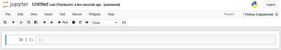
• A new tab will open with an empty notebook. You’ll see an interface with a blank code cell labeled something like In [ ]:

• Rename the notebook (optional). By default, it’s “Untitled”. To name it, click on the title at the top (Untitled.ipynb) and type a new name, then click Rename.

• Save the notebook periodically by clicking the save icon (or pressing Ctrl + S). Notebooks autosave periodically, but it’s good to save often.

Dashboard → New → Python 3 will open a fresh notebook. The new .ipynb file appears in the dashboard’s file list (with a green “Running” tag) when it’s open as shown below.

The Notebook Interface

Inside an open notebook (in its browser tab), you’ll see the notebook interface. It has several key parts:

• Title Bar: At the top left is the notebook’s title (e.g., “Untitled”). Click here to rename.

• Menu Bar: Below the title is the menu (File, Edit, View, Insert, Cell, Kernel, Widgets, Help). Each menu has many options (e.g., File → Save, Cell → Run All).

• Toolbar: Below the menu is a row of icons (save, add cell, cut/copy/paste cells, move cells up/down, run, interrupt, restart, etc.). These are quick-action buttons.

• Notebook Area: This is the main scrollable area containing cells. Each cell can be code or Markdown. Cells are executed one at a time.

Figure: A Jupyter notebook showing a Markdown Cell (top) and a Code Cell (bottom). Code cells (with In [ ]:) let you write and run code. Markdown cells let you write formatted text, lists, or equations. Here, the left border color (blue) indicates the notebook is in Command mode.

• Code Cells: Used for writing Python code. When you run a code cell, Jupyter sends it to the kernel, which executes it and displays the output (text or graphics) below the cell. The default cell type is Code.

• Markdown Cells: Used for writing rich text using Markdown (plain text syntax that can include headings, lists, links, images, and LaTeX math). When you “run” a Markdown cell, Jupyter renders the formatted text. This is how you add explanations, section titles, or equations to your notebook.

You can switch a cell’s type via the toolbar menu or keyboard shortcuts. For example, to convert a cell to Markdown, select it and press M (in Command mode). To convert back to code, press Y. Use Markdown cells to document your steps, describe results, or write math equations.

Edit Mode vs Command Mode

Jupyter uses a modal interface: Edit Mode and Command Mode. The mode determines what your keystrokes do.

• Edit Mode (green border): Click inside a cell (or press Enter when a cell is selected) to enter edit mode. The cell’s border turns green, and you can type/edit code or text in the cell. In Edit mode, your keystrokes (letters, numbers) go into the cell content as usual.

• Command Mode (blue border): Press Esc (or click outside the cell editor) to enter command mode. The cell’s border turns gray/blue. In Command mode, you cannot type into the cell; instead, keypresses perform notebook-level commands (like copying or adding cells). For example, when the cell border is blue, pressing C will copy the cell (see keyboard shortcuts below).

The color of the cell border indicates the mode: green for edit, blue/gray for command. You can always toggle modes: press Esc to go to Command mode, Enter to go to Edit mode on the selected cell.

Running Cells and Keyboard Shortcuts

• Run a Code Cell: Press Ctrl + Enter to run the selected cell and stay on it. Press Shift + Enter to run the cell and move the cursor to the next cell (creating a new cell below if necessary). There is also Alt + Enter, which runs the cell and inserts a new cell below.

• New lines vs Execution: Pressing Enter (in Edit mode) just inserts a new line in the cell (without running). Only Shift+Enter or Ctrl+Enter will execute the cell.

• Interrupt/Restart: If the code is taking too long, you can stop it via the stop button or Kernel → Interrupt. To reset the Python kernel, use Kernel → Restart (this clears all variables).

• Run All: Use Cell → Run All (or Kernel → Restart & Run All) to execute all cells from top to bottom.

Essential keyboard shortcuts: (These work when in Command mode – press Esc first if needed.)

• A → Insert a new cell above the selected cell.

• B → Insert a new cell below the selected cell.

• C → Copy the selected cell.

• X → Cut (delete) the selected cell to the clipboard.

• V → Paste the cell from the clipboard below the current one.

• D, D (press D twice) → Delete the selected cell.

• M → Convert the current cell to Markdown.

• Y → Convert the current cell to Code.

• Z → Undo the last cell operation (e.g., deletion).

These shortcuts let you add, move, and remove cells quickly without touching the mouse. For example, to build a notebook, you might insert a Markdown cell with a heading (A or B, then M to make it Markdown) and then below it a code cell (Y to set type) to run code.

Best Practices for Beginners

• Use Many Small Cells: Break your work into multiple small cells rather than one giant block of code. This improves readability and makes debugging easier. You can run and test each part separately. As one guide notes, it’s better to divide the analysis into “smaller chunks” across cells and even multiple notebooks.

• Document with Markdown: Use Markdown cells to explain your steps and results. Clear comments and text help others (and yourself later) understand the notebook.

• Sequential Execution: Especially before sharing, restart the kernel and use “Run All” to ensure the notebook runs top-down without errors. This catches hidden dependencies on previously run cells.

• Save Outputs: If an analysis step is slow, consider saving its output to a file or variable so you don’t have to recompute it every time.

• Parallel Work: Each notebook you open runs in its own Python kernel. You can open and run multiple notebooks in parallel if you like (each one will have a “Running” tag in the dashboard). This means unrelated tasks can be in separate notebooks and executed concurrently. For example, you could run data-cleaning code in one notebook while exploring plots in another. Keeping tasks separate helps avoid confusion and leverages multiple cores if your machine allows it.

By following these steps and using the interface effectively, you’ll be able to leverage Jupyter Notebook for interactive data analysis and automation.