
Get Hired: A Financial Derivatives Interview Handbook
- Feb 23, 2022
- 31 min read
Updated: Mar 16, 2024
Congratulations! You've landed an interview I understand, and now it's time to prepare for it!
One of the most important guides at your disposal is this interview guide. think of it as your roadmap to success, guiding you through the twists and turns of the interview process. Here's how to decode and utilize this essential document effectively.

Start by carefully reading through this interview guide from start to end. Pay attention to any instructions, formatting, or specific questions provided.
Spend time on each topic, take notes, strive for understanding, and, most importantly, attempt to model these complex problems using either Excel or Python.
While this interview guide provides a detailed framework, be prepared to adapt and think on your feet. Interviewers may ask unexpected or follow-up questions to test deeper into certain areas.
After the interview, reflect on your performance and seek feedback from trusted sources, such as mentors, career advisors, or interview coaches. Again, take notes of areas of improvement and incorporate them into your preparation for future interviews.
What are the different types of Derivative instruments in the market?
Derivatives are financial instruments whose value is derived from the value of an underlying asset, index, or rate. They are primarily used for hedging risks, speculation, or arbitrage. There are several types of derivatives traded in the market:
Forward Contracts: These are customized contracts between two entities, where settlement takes place on a specific date in the future at a price agreed upon today.
Futures Contracts: These are similar to forward contracts but are standardized and traded on a futures exchange. They obligate the buyer to purchase an asset (or the seller to sell an asset) at a predetermined future date and price.
Options: Options are contracts that give the holder the right, but not the obligation, to buy or sell an underlying asset or instrument at a specific strike price on or before a specific date. There are two primary types: Call Option: Gives the holder the right to buy an asset at a specified price. Put Option: Gives the holder the right to sell an asset at a specified price.
Swaps: Swaps are agreements between two parties to exchange sequences of cash flows for a set period. The most common type is the interest rate swap, where one party agrees to pay a fixed interest rate in exchange for receiving a floating interest rate from another party.
Credit Derivatives: These are designed to transfer credit risk between parties. The most common type is the Credit Default Swap (CDS), where one party will pay another in the event of a credit event like a default.
Structured Products: These are complex instruments, often used in the over-the-counter (OTC) market, that are derived from a single security, a basket of securities, options, indices, commodities, debt issuances, or foreign currencies.
Warrants: These are similar to options and provide the holder the right but not the obligation to purchase securities (usually equity) from the issuer at a specific price within a certain time frame.
Exotic Derivatives: These are more complex derivatives which might include features such as knock-in or knock-out barriers, lookback options, Asian options, etc. They often have conditions not found in standard options or other derivative products.
Caps and Floors: These are types of interest rate derivatives where the buyer receives payments at the end of each period when the interest rate exceeds (in the case of a cap) or is below (in the case of a floor) a specified fixed rate.
Collars: An interest rate collar is the simultaneous purchase of an interest rate cap and sale of an interest rate floor on the same index for the same maturity and notional principal amount.
What are options in the derivatives market?
An option is a contract between the contracting parties to buy-sell an underlying asset at a pre-determined price (known as the strike price) for a pre-determined quantity (known as contracts having lot size) on a pre-determined later date (known as maturity/expiry date). A buyer of an option has a right to buy (in case of a call option) or sell (in case of a put option) but not an obligation to do so, and therefore, options are a non-linear product.
A call option is a derivative contract that gives the right to the buyer, to buy an underlying asset at a pre-determined price (called the strike price) having a pre-determined quantity (called lot size) on a pre-determined later date (called maturity or expiry date). However, it does not obligate the buyer to do so.

A put option is a derivative contract that gives the right to the buyer, to sell an underlying asset at a pre-determined price (called the strike price) having a pre-determined quantity (called lot size) on a pre-determined later date (called maturity or expiry date). However, it does not obligate the buyer to do so.
How a call option can be used in the financial market?
One common use of call options is to hedge against market increases. By purchasing call options, an investor can protect their portfolio against potential losses in the event that the underlying asset increases in value.
Call options can also be used to generate income through the sale of call options. When an investor sells a call option, they collect a premium from the buyer in exchange for the obligation to potentially sell the underlying asset at a later date.
Call options can also be used to speculate on market movements. For example, an investor who believes that the price of an underlying asset will increase in the future may purchase call options as a way to profit from the potential price increase.
How a put option can be used in the financial market?
One common use of put options is to hedge against market declines. By purchasing put options, an investor can protect their portfolio against potential losses in the event that the underlying asset declines in value.
Put options can also be used to generate income through the sale of put options. When an investor sells a put option, they collect a premium from the buyer in exchange for the obligation to potentially buy the underlying asset at a later date.
Put options can also be used to speculate on market movements. For example, an investor who believes that the price of an underlying asset will decline in the future may purchase put options as a way to profit from the potential price decline.
What are the differences between hedging, speculation, and arbitrage?
Hedging involves making investments with the aim of minimizing the risk of unfavorable price fluctuations/movements in an asset and taking offsetting positions in related securities. While hedging can reduce potential risks, it also limits potential gains. Hedging through options and futures contracts are available for nearly every type of investment, including those involving stocks, interest rates, currencies, commodities, and other non-financial instruments.
Speculation could be a trading strategy based on predictions of market trends. Speculators make calculated guesses about the future price movements of securities and trade accordingly. They may bet against market movements to make profits from price fluctuations. Speculation is inherently risky, and speculators are exposed to both the upside and downside of the market. In contrast to hedgers, who prioritize risk reduction, speculators prioritize the potential for profit.
Arbitrage refers to the practice of simultaneously buying and selling an asset in different markets to capitalize on price discrepancies. It is a short-term strategy that exploits inefficiencies in the market. Although such opportunities are transitory, they can arise in currency and stock trading across multiple exchanges.
What are the sensitivities to an option derivative instrument?
Option sensitivities are the tools that measure how an option's price/premium is affected by the change in underlying parameters on which the value of the option depends. Each greek value measures the sensitivity of an option to a small change in a specific underlying parameter. The most common greeks are-
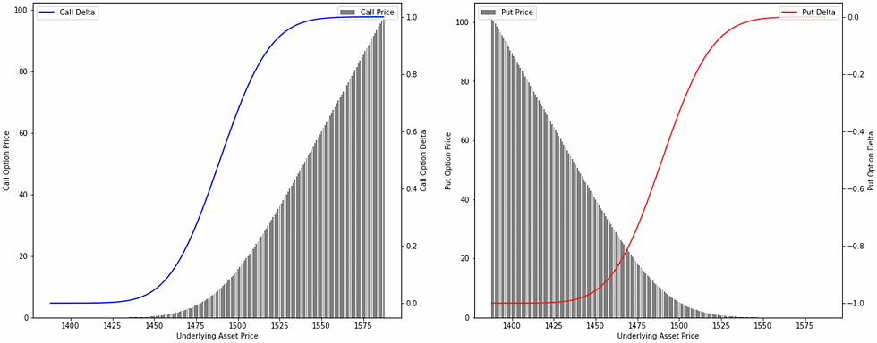
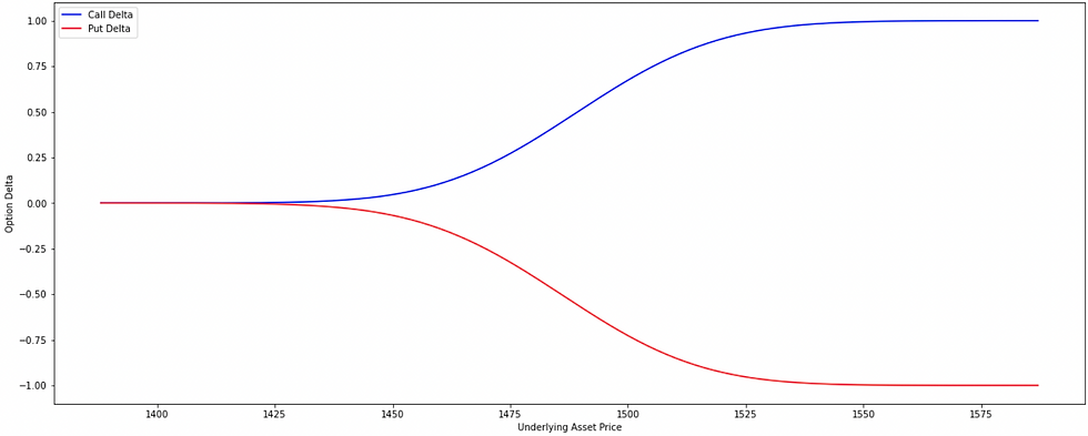
Delta is a rate of change in the price of an option with respect to a change in the price of the underlying asset, other factors being constant. In other words, an option's delta is an amount by which the price of an option is expected to change with respect to a $1 change in the price of the underlying asset, other factors being constant. If the price of an underlying asset increases, the option delta of both call and put options increases too. The delta of a call option always remains positive (it will range between 0 and 1, representing a positive relationship with the underlying) and the delta of a put option always remains negative (ranging between -1 to 0, representing a negative relationship with the underlying). 'delta' sensitivity is important because it helps, (1). traders estimating the movement in the price of an option for any change in the price of the underlying asset. (2). risk managers to gauge the directional risk and being the most crucial risk attribute for analysis though it explains the first-order risk only.
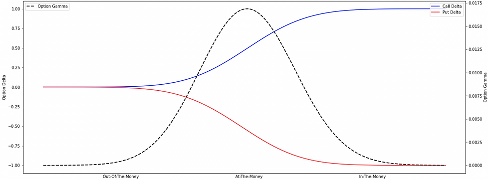
Gamma is a rate of change in the option's delta with respect to a change in the price of the underlying asset, other factors being constant. In other words, an option's gamma is an amount by which the option's delta is expected to change with respect to a $1 change in the price of the underlying asset, other factors being constant. Gamma influences the delta of calls and puts in the same direction and gamma is always positive for long and negative for short. 'gamma' sensitivity is important because it helps, (1). traders to estimate the movement in the option's delta for any change in the price of the underlying asset. (2). risk managers to gauge the directional risk add-on to the first-order risk and is the most crucial risk attribute for analysis as it explains the second-order risk, sometimes referred to as higher-order risk.
Understanding Vega: A Deep Dive into Options Greek
Vega is a rate of change in the price of an option with respect to a change in the volatility of the underlying asset, other factors being constant. In other words, an option's vega is an amount by which the price of an option is expected to change with respect to a 1% change in the volatility of the underlying asset, other factors being constant. If the volatility of the underlying asset increases, the vega of both call and put options increases too. It is important because it helps traders and risk managers to estimate the potential impact of changes in volatility on an option's price. Vega is typically represented as a positive number.
Understanding Theta: A Deep Dive into Options Greek
Theta is a rate of change in the price of an option with respect to a change in the time remaining until expiration, other factors being constant. In other words, an option's theta is an amount by which the price of an option is expected to change with respect to a one-day decrease in the time remaining until expiration, other factors being constant. If the time remaining until expiration decreases, the theta of both call and put options increases. It is important because it helps traders and risk managers to estimate the potential impact of time decay on an option's price. Theta is typically represented as a negative number.
Understanding Rho: A Deep Dive into Options Greek
Rho is a rate of change in the price of an option with respect to a change in the interest rates, other factors being constant. In other words, an option's rho is an amount by which the price of an option is expected to change with respect to a 1% change in interest rates, other factors being constant. If the interest rates increase, the rho of both call and put options increase for long positions and decrease for short positions. It is important because it helps traders and risk managers to estimate the potential impact of changes in interest rates on an option's price. Rho is typically represented as a positive or negative number, depending on whether the option is a call or put and whether it is long or short.


What is the moneyness of an option?
The moneyness of an option can be of three types:
In-the-money (ITM) options: A call option is considered to be ITM when its underlying asset price is trading above its strike price. A put option is considered to be ITM when its underlying asset price is trading below its strike price.
Out-of-the-money (OTM) options: A call option is considered to be OTM when its underlying asset price is trading below its strike price. A put option is considered to be OTM when its underlying asset price is trading above its strike price.
At-the-money (ATM) options: A call and a put option are considered to be ATMs when their underlying asset price is equal to their strike price.
What would be the delta of a put option if the delta of a call option is 0.7?
(assuming that the underlying asset is a: dividend-paying stock, non-dividend-paying stock)
Explain the behavior of a delta curve w.r.t moneyness.
Explain the behavior of a delta w.r.t volatility.
Traders become more conscious when the volatility in the market rises as they perceive an increased likelihood that the ITM strike option could land OTM at expiration and therefore, the probability (i.e. delta) of an option landing ITM diminishes. In other words, low implied volatility will tend to have a higher delta value for ITM options because the probability of an ITM option landing ITM is high and a lower delta value for OTM options because the probability of an OTM option landing ITM is very low.

Therefore, if the implied volatility increases, the delta of OTM options will also increase while that of ITM options will decrease. And if the implied volatility decreases, the delta of OTM options will also decrease while that of ITM options will increase.

Understand how option Delta and Gamma of call and put options react to changing volatilities.
In my opinion, understanding delta and gamma in relation to moneyness offers valuable information, it's crucial to also consider the effects of volatility and time decay. these elements play a significant role in shaping option pricing dynamics and various strategies which are being applied.
(to really see this in action, attached a video having 4 different plots. It will paint a clearer picture than just words can.)
Explain the behavior of a delta curve w.r.t time-decay.
(short-dates vs. long-dated options)

Explain the behavior of a gamma curve w.r.t moneyness.

Explain the behavior of a gamma w.r.t volatility.

Explain the behavior of a gamma curve w.r.t time-decay.
(short-dates vs. long-dated options)

Do you think that option's vega can be negative in any case? If yes, what could be that scenario?

What are the assumptions of the Black-Scholes-Merton (BSM) Model for pricing options?
The underlying asset price follows a Geometric Brownian Motion (GBM), which means, the underlying price follows Log-Normal Distribution. And therefore, LN(St/St-1) i.e., continuous returns on the stock price follows Normal Distribution.
As mentioned, the Geometric Brownian Motion (GBM) implies continuous value i.e., there are no jumps in the share price.
Volatility in the underlying asset is known and constant and is not changing (throughout the option period).
The annualized continuously compounded dividend yield on the underlying is known and constant throughout the option period.
Since BSM Model is an analytical closed-form solution to price an option, and therefore, it can be only applied to European options as it can be exercised only on the expiration date.
Markets are frictionless (i.e., there are no transaction costs, no taxes, and no regulatory constraints such as no restrictions on short selling with full use of proceeds and continuous trading available).
Markets are efficient (i.e. no-arbitrage opportunity available and the underlying asset is liquid).
The annualized continuously compounded risk-free interest rate is constant throughout the option period the same is applicable for both- unlimited lending and borrowing.
What are the factors /model inputs that determine the price of an option?
The Black-Scholes-Merton (BSM) Model for pricing options is based on six inputs:
Underlying Price: the current market price of the underlying asset on which the option is based. This can be a stock, a commodity, an index, or any other financial asset.
Strike Price: the price at which the option can be exercised by the holder.
Volatility: the measure of the amount by which the price of the underlying asset is expected to fluctuate over a given period of time.
Time to Expiration: the length of time remaining until the option expires. This is typically measured in days, weeks, or months.
Interest Rate: the prevailing risk-free interest rate, which is used to calculate the present value of future cash flows.
Dividend Yield: the expected dividend yield of the underlying asset, which is also used to calculate the present value of future cash flows.
By inputting these six variables into the BSM formula, one can estimate the fair value of an option.

What is the use of the Binomial Model if we have the Black-Scholes-Merton (BSM) Model for pricing options?
One advantage of using a binomial model over the BSM model is that it can price path-dependent options. It is primarily used to price American and Bermudan options because of the feature that it can be exercised prior to expiration, unlike the BSM model which cannot check at what point it can be exercised, and therefore, the binomial model is the only recourse.

What is the composition of the option's price /premium?
Option’s price has two components – Intrinsic Value & Extrinsic Value. Extrinsic value has further two components – Time Value & Volatility Premium.

Intrinsic Value: It is the value by which the option is ITM. It is always positive, it cannot be negative. The options that are OTM or ATM have zero intrinsic value. Intrinsic value is exposed to the directional risk or we can say that the moneyness directly impacts the intrinsic value of an option and the sensitivity to measure the risk is via option’s Delta and Gamma.
In the case of-
call options, Intrinsic Value = Max[Underlying Price – Strike Price, 0]
put options, Intrinsic Value = Max[Strike Price – Underlying Price, 0]
Extrinsic Value: It is the excess that market participants are ready to pay for an option over and above its intrinsic value. In the case of both call and put options, Extrinsic Value = Actual Option Price – Intrinsic Value. It further has two components-
Time Value: The sensitivity to measure the time decay is the option’s Theta.
Volatility Premium: The sensitivity to measure the volatility risk is the option's Vega.
What are N(d1) and N(d2) /model features in the BSM formula?
N(d1) is the probability that determines the expected payoff in case the option is getting exercised in the risk-neutral world, and therefore, the expression [ S(0) * N(d1) * e^rt ] in the equation is the expected stock price at expiration date (S(0)*e^rt) calculated using the probability (N(d1)) in a risk-neutral world.
On the other hand, the exercise/lapse is dependent on the moneyness of an option, and therefore, the strike price (K) is only transacted if the option is ITM standing on the expiration date whose probability is N(d2)- represented by [ K * N(d2) ].

What are the limitations of the BSM Model?
The underlying share price assumed to be following Geometric Brownian Motion (GBM) implies a random walk, and therefore, large jumps are not incorporated in the model. However, emerging countries or companies that are going into some major corporate events like mergers, etc. exhibit jumps in the share price, and therefore, BSM should not be applicable in such cases.
Volatility in the underlying asset is assumed to be constant throughout the option period, but the volatility is dynamic in real life. The implied volatility calculated by reverse engineering using BSM Model is generally greater than the expected volatility derived from the historical data of the underlying and is changing over time.
The BSM formula nowhere considers dividends distributed during the option period, and thus, not correctly price an option.
Frictionless markets do not exist in reality. Therefore, transaction costs, taxes, and regulatory constraints come into play.
What is the Taylor-Series Approximation /Expansion technique? & How it can be used in pricing options?
When it comes to valuing any financial product or any derivative instrument, the first thing that comes into our mind is its pricing function. However, it is not always feasible to go for a full valuation model which involves its pricing function. It is time-consuming, the system should be efficient enough to capture a large number of trades, and the model should be precise enough to calculate the price accurately.
Instead, one can use the "Taylor Series Approximation/Expansion" technique which helps us price/value any financial product or derivative instrument on the basis of its sensitivities. Those sensitivities could be "duration-convexity” or "delta-gamma" depending upon the type of financial product or derivative instrument we are dealing with. The approach for calculating the same is pretty simple. It captures all the order movements separately (first-order, second-order, and higher-order) and the sum total of these movements together with the base price will get us the changed price.
Taylor's function =f(a)+f′(a)(x−a)+f′′(a)/2!(x−a)^2+f′′′(a)/3!(x−a)^3+.....
However, mathematically, it is a very demanding process to capture the slope of a non-linear price function, especially for structured and path-dependent instruments. Even after capturing the partial derivatives, we're still left with the error from Taylor's approximation. It seems that the error increases with the increased market move in the underlying risk factor(s).

With the limitations of Taylor's approximation/expansion technique and considering the computing power of full valuation models in today's generation, full valuation of each and every trade even under different scenarios could be more advantageous/accurate than having to defend the assumptions underlying the Taylor approximation.
What is the difference between a Monte Carlo simulation and a finite difference method for pricing options?
A Monte Carlo simulation and a finite difference method are two different techniques used for pricing options in financial modeling. The key differences between these methods are as follows:
Monte Carlo Simulation: Monte Carlo simulation is a statistical method used to model the behavior of a system or process by generating random variables that simulate the underlying probability distributions. In the context of option pricing, Monte Carlo simulation involves generating a large number of random paths for the underlying asset price and computing the payoff of the option at each path. The average of the payoffs over all the paths is used to estimate the option price.

Finite Difference Method: The finite difference method is a numerical technique used to solve partial differential equations. In the context of option pricing, the Black-Scholes equation is a partial differential equation that can be solved using the finite difference method. The method involves dividing the time and price domain into a grid and approximating the derivatives of the option price with respect to time and price using finite differences. The resulting system of equations can be solved iteratively to obtain the option price.
What is Implied Volatility (IV)? And how is it computed?
Implied volatility is the market's consensus of a likely movement in an underlying price. It is one of the determinants of pricing options. The real/actual prices of options trading in the market do not follow the BSM Model- not the constant volatility assumption. The actual prices have more variability than the volatility assumed by the BSM Model and that's the main reason why we compute volatility implied by the actual option's price.
The methodology behind modeling the implied volatility is that we take the actual option price determined by the demand and supply in the market at which the trades are settled and then use BSM Model to reverse engineer by iterating the volatility until the model equates to the model price with the actual price. The volatility at which the model equates the model price with the actual option price is implied volatility.

Explain the behavior of an implied volatility curve w.r.t moneyness.
As stock price increases, the ATM strike put option becomes OTM. This will lead to generating more put option contracts at OTM strike (act as insurance) and hence, higher demand and higher implied volatility. This means implied volatility is positively related to the underlying price. In other words, as stock price increases, the implied volatility also increases for a particular strike price, implied volatility curve shifts to the right resulting in instability and seems to depend upon the moneyness of the option.
Explain the behavior of an implied volatility curve w.r.t time-decay
(short-dated vs. long-dated options)
The implied volatility computed by reverse engineering using BSM Model, a pronounced curvature is formed and that curvature is more pronounced for short-dated options and less pronounced for long-dated options. This is based on the fact that long-dated options have more time value (the difference between the actual option price and the intrinsic value of that option), while short-dated options have less time value-priced in them. Also, the properties of log-normal distribution are, that there should not be any price jumps (caused due to corporate events, financial budget, etc.) that directly impact an option's intrinsic value. But, it tends to average out in the long run and that is why we see a smooth-flattish implied volatility curve for long-dated options.
What is implied volatility skew & smile? &
Why implied volatility is not constant in the real world?
A plot of the implied volatility of an option across different strike prices is known as the volatility skew. Why? -- The options with the same underlying, and same expiry but with different strike prices have different implied volatility (it is not the same). Two particular volatility skew patterns are- volatility smile and volatility smirk (and that could be reverse skew or forward skew).
A Volatility Smile pattern is generally seen for options in the forex/currency market. It represents that the demand (or implied volatility) is higher for options that are ITM and OTM i.e., lower and higher strike price options.
On the other hand, a Volatility Smirk:
Reverse Skew is seen for options in the equity market and index options. In a reverse skew pattern, the implied volatility is comparatively higher for lower strike price options than the higher strike price options. This suggests that OTM put options and ITM call options are more expensive having greater demand than the ITM put options and OTM call options respectively. The reason is- crash-o-phobia and leverage.
Volatility Smirk- Forward Skew is seen for options in the commodity market. In the forward skew pattern, the implied volatility is comparatively higher for higher strike price options than the lower strike price options. This suggests that ITM put options and OTM call options are more expensive having greater demand than the OTM put options and ITM call options respectively. the reason is- fear of business shutdown.
What is the difference between a local volatility model and a stochastic volatility model?
The local volatility model and stochastic volatility model are two widely used approaches in quantitative finance for pricing financial derivatives. The key difference between the two lies in the way they handle volatility.
A local volatility model assumes that the volatility of the underlying asset is a deterministic function of time and the asset price, meaning that the volatility is fixed and does not change with time or the asset's price. This makes local volatility models computationally less complex than stochastic volatility models. However, they are less accurate in modeling the behavior of the underlying asset, particularly in extreme market conditions.
this model would be more appropriate to use in the case of:
European plain vanilla options with no early exercise features.
When market volatility is stable and not subject to large swings.
When pricing a single asset or a portfolio of assets with similar risk characteristics.

A stochastic volatility model assumes that the volatility of the underlying asset is a random variable that follows a particular stochastic process. Stochastic volatility models are more complex and computationally intensive, but they can better capture the behavior of the underlying asset, particularly in volatile market conditions.
this model would be more appropriate to use in the case of:
American-style options or other options with early exercise features.
When the market volatility is highly volatile and unpredictable.
When modeling the behavior of complex derivatives that depend on multiple underlying assets with different risk characteristics.

What is delta-hedging?
Delta hedging aims to reduce the linear risk associated with the underlying price movement by an offsetting approach of long-short positions. The relationship between the change in the price of an option and the change in the price of an underlying is called the hedge ratio and that can be used to hedge a delta-risky position to remain delta-neutral.
For example, a short call option position can be delta hedged by taking a long position via underlying stock or by taking a long call position keeping other factors on mute to remain delta-neutral. Of course, continuous rebalancing would be required as the delta keeps changing due to moneyness, volatility, and overtime.
Why delta rebalancing is required to remain delta-hedged or delta-neutral?
Delta hedging is a continuous process (as the delta is changing due to a change in the underlying price, the position is momentarily delta-neutral) and should be performed throughout the tenure of an option. Delta hedging can’t be done by taking a static position but it requires dynamic rebalancing.
However, increasing the frequency of rebalancing reduces the overall volatility but at the expense of increased commissions which might not be as profitable as compared to holding till the expiration date for retail traders. Hence, delta rebalancing is a great hedge against directional risk at the same time the frequency of rebalancing is also an active decision to be taken properly.

What is delta-gamma-hedging?
Delta-Gamma hedging is a hedging technique that aims to reduce the linear as well as the non-linear risk associated with the underlying price movement to some extent by an offsetting approach of long-short positions. The risk is associated with the direction and both greeks- delta and gamma measure the sensitivity of the directional change.
Basically, it combines a delta hedge and a gamma hedge to remain delta-gamma-neutral. Using a gamma hedge in conjunction with a delta hedge requires a trader to create an additional hedge when the delta changes. And therefore, continuous rebalancing would be required as delta and gamma keeps changing due to moneyness, volatility, and over time.

What is a long straddle? &
How is it different from a long strangle?
(also prepare for: short straddle, and short strangle)
A long straddle is an options trading strategy that involves purchasing both a call option and a put option at the same strike price and expiration date. The idea behind a long straddle is to profit from significant price movements in the underlying asset, regardless of whether the price goes up or down.
When a trader buys a long straddle, they pay a premium for both the call and put options. The maximum loss for this strategy is limited to the total premium paid for both options. However, the potential profit is theoretically unlimited, as the trader can profit from large price movements in either direction.
The long straddle strategy works best when there is expected to be significant volatility in the underlying asset, but the direction of the price movement is uncertain. If the price of the underlying asset moves significantly in either direction, the value of either the call or put option will increase, while the other option will expire worthless. The trader can then sell the profitable option and potentially make a profit that exceeds the premium paid for both options.
On the other hand, a long strangle involves buying a call option and a put option with different strike prices, but with the same expiration date. The strike price for the call option is typically higher than the strike price for the put option. This means that the trader is betting on significant price movements in either direction, but they believe that the price will move more in one direction than the other. The maximum loss for a long strangle is also limited to the total premium paid for both options, but the potential profit is less than that of a long straddle because the price must move more significantly in one direction to make a profit.
What is the risk associated with using a long-straddle trading strategy?
A long straddle can be a high-risk strategy, as
it requires significant price movements in either direction to be profitable.
the passage of time can erode the value of both options, which can result in significant losses if the underlying asset does not move enough to offset the time decay.
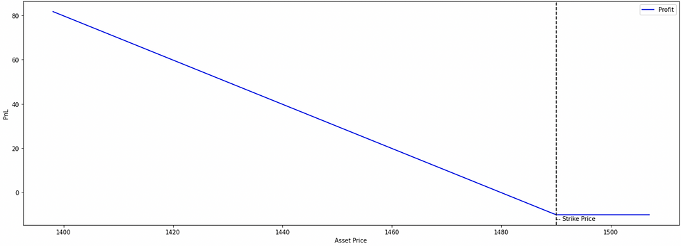
Can you explain the payoff-profit profile of a long straddle?
(also prepare for: short straddle, long strangle, and short strangle)
Can you explain the risk profile of a short strangle in terms of greeks? or
Can you explain the gamma profile of a short strangle?
(also prepare for: long strangle, long straddle, and short straddle)
Can you explain the gamma profile of a 100-110 bullish call spread? or
When will you lose the maximum on gamma if the position is a 100-110 bullish call spread?
(also prepare for: bearish call spread, bearish put spread, and bullish put spread)
Highlight the differences between a forward and a futures contract.
forward contracts are agreements entered into by two parties (buyer and seller) to trade an asset at some future date at an agreed price/rate while futures contracts are agreements entered by a party (buyer or seller) with an Exchange with standardized terms.
forward contracts are traded over the counter (negotiated) between two parties while futures contracts are traded on the Exchange platform where one party is the buyer/seller and the other is the exchange.
forward contracts are non-standardized contracts where the terms such as forward price/rate, lot size, maturity date, asset quality, etc. are agreed upon between both parties while futures contracts are highly standardized.
forward contracts are settled on the maturity date, the date agreed upon by both parties in the contract, usually with physical delivery while future contracts are settled on a daily basis, and that too mark-to-market cash.
theoretically, forward contracts have no requirement to post collateral at any point while futures contracts require a margin at initial, some maintenance margin, and a variation margin.
Can you explain the impact of interest rate changes on forwards and futures contracts?
How would you explain the impact of interest rate changes on a forward contract and a futures contract, and how does the position held in the contract (long or short) and the direction of the interest rate change (increase or decrease) affect the benefit?
The impact of interest rate change depends on the position held in the contract, whether long or short, and whether the change in interest rate is favorable or unfavorable to the position.
Forwards:
If interest rates decrease, the holder of a long position (i.e., the buyer) in a forward contract may benefit as the cost of borrowing to finance the purchase of the underlying asset may be lower.
If interest rates increase, the holder of a short position (i.e., the seller) in a forward contract may benefit as the income earned from lending the proceeds from the sale of the underlying asset may be higher.
Futures:
If interest rates decrease, the party with a negative mark-to-market value will benefit as they will be able to finance the margin requirement at a lower cost.
If interest rates increase, the party with a positive mark-to-market will benefit as they will earn more on the funds held in the margin or paid out.
What are Interest-Rate Swaps (IRS)?
Interest-rate swaps (IRS) are financial derivatives in which two parties agree to exchange one stream of cash flows for another, based on a specified principal amount. These cash flows are typically based on a fixed interest rate and a floating interest rate. IRS is used to hedge against interest rate risk or to speculate on changes in interest rates. They can be used by businesses, governments, and individuals to manage their exposure to interest rate fluctuations.
In an interview, it would be helpful to provide an example of how an IRS works and the benefits it provides to the individual parties involved.
Let's say that a company, Company A, has issued a bond with a fixed interest rate of 5%. However, Company A is worried that interest rates may increase in the future, which would increase its debt servicing costs. To hedge against this risk, Company A can enter into an IRS with a financial institution, where they agree to pay a fixed rate of 5% on a certain principal amount and receive a floating rate in return. This allows Company A to lock in a fixed interest rate and protect itself against any increases in interest rates.
On the other hand, the financial institution is speculating that interest rates will decrease, so they agree to pay a floating rate and receive a fixed rate of 5% in return. If interest rates do decrease, the financial institution will benefit from paying a lower rate than what they are receiving.
In this example, both parties have benefited from the IRS. Company A has protected itself against interest rate risk and the financial institution has the opportunity to profit from a decrease in interest rates. This is the main benefit of the IRS, it helps to manage interest rate risk.
What are Mortgage-Backed Securities (MBS)?
Mortgage-Backed Securities (MBS) are financial products that are created when a large number of individual mortgages are pooled together and then sold to investors. The cash flow from the individual mortgage payments is then used to pay back the investors who hold the MBS.
MBS can be issued by a variety of entities, including government-sponsored enterprises such as Fannie Mae and Freddie Mac, as well as private financial institutions. MBS are typically classified as either agency MBS or non-agency MBS, depending on the entity that issued them.
Agency MBS are backed by the full faith and credit of the U.S. government, which means they are considered to be relatively safe investments.
Non-agency MBS, are not guaranteed by the government and may carry a higher level of risk.
Investors in MBS can receive a regular stream of income in the form of interest payments, as well as potential capital appreciation if the value of the underlying mortgages increases over time. However, as with any investment, MBS carries some level of risk, including the possibility of default by the borrowers on the underlying mortgages.
How Residential Mortgage-Backed Securities (RMBS) are different from Commercial Mortgage-Backed Securities (CMBS)?
Residential Mortgage-Backed Securities (RMBS) and Commercial Mortgage-Backed Securities (CMBS) are both types of Mortgage-Backed Securities (MBS), but they differ in several ways.
RMBS are backed by residential mortgages, which are typically used to purchase single-family homes or other residential properties. On the other hand, CMBS are backed by commercial mortgages, which are used to finance commercial properties such as office buildings, shopping centers, and hotels.
the underwriting and risk assessment processes for RMBS and CMBS are different. RMBS typically involves evaluating the creditworthiness of individual borrowers, while CMBS focuses more on the creditworthiness of the property and its potential cash flow. This is because commercial properties often have multiple tenants and sources of income, while residential properties typically have a single occupant and income source.
the performance of RMBS and CMBS can be affected by different economic factors. For example, the performance of RMBS is often closely tied to the overall health of the housing market and the economy, while the performance of CMBS can be more sensitive to factors such as changes in interest rates, tenant occupancy rates, and the strength of the local real estate market.
What are Credit Default Swaps (CDS)? or
How Credit Default Swaps (CDS) can be used in mitigating default risk?
What are Credit Debt Obligations (CDO) and CDO-Squared?
-- more getting added --
Important Terminologies
let's focus on terminologies for Financial Derivatives!
Basic Derivative Instruments
Forward Contract: A non-standardized contract to buy or sell an underlying asset at a specified future date for a price agreed upon today.
Futures Contract: A standardized forward contract traded on an exchange, obligating the buyer to purchase and the seller to sell the agreed-upon quantity of an underlying asset at a set price.
Option: A contract that offers the buyer the right, but not the obligation, to buy (call) or sell (put) an underlying asset or instrument at a set strike price.
Swap: An agreement between two parties to exchange sequences of cash flows. Common types include interest rate swaps and currency swaps.
Risk and Valuation Concepts
Intrinsic Value: The difference between the underlying asset's price and the strike price of the derivative, if favorable; otherwise, it's zero. It represents the immediate cash value of the option if it were exercised.
Time Value: The difference between the option's premium and its intrinsic value. Time value reflects the potential for future changes in the option’s value and decreases as the expiration date approaches.
Implied Volatility: The volatility of the underlying asset derived from the option's price. It reflects market expectations of future price fluctuations, often used in option pricing models.
Delta: Measures the sensitivity of an option's price to changes in the price of the underlying asset. It can be interpreted as the expected change in option value for a $1 change in the underlying.
Gamma: Measures the rate of change in the option's delta for a unit change in the underlying asset. It's crucial for assessing the stability of the delta as the market moves.
Vega: Indicates how the option's price reacts to changes in the volatility of the underlying asset. It's crucial for those trading volatility strategies.
Theta: Represents the rate of change of an option's price concerning time. Often referred to as time decay, it quantifies how much value an option loses as one day passes.
Rho: Measures the sensitivity of option value to changes in the interest rate. Important for longer-dated options where interest rate shifts can have a more pronounced effect.
Vomma (or Volga): Measures the rate of change in Vega for a change in implied volatility. It's a second-order Greek that provides insight into the convexity of the Vega.
Speed (or Color): Measures the rate of change in Gamma for a change in the underlying asset price. It gives traders a deeper view of how Gamma and Delta might change as the market moves.
Charm (or Delta Bleed): Measures the rate of change in Delta over the passage of time. It's useful for understanding how the Delta might evolve as days pass.
Counterparty Risk: The risk that the other party in a derivative contract will not live up to its contractual obligations. It's especially concerning in over-the-counter markets where contracts aren't standardized.
Black-Scholes Model: A mathematical model used to price European-style options. Developed by Fischer Black, Myron Scholes, and Robert Merton, it's foundational in modern financial theory.
Binomial Option Pricing Model: Uses a lattice-based model to value options, accommodating various changes in parameters over time. It provides a more flexible framework compared to Black-Scholes but can be more computationally intensive.
Liquidity Risk: The risk that a derivative cannot be sold or bought quickly enough because of a lack of market participants or disruptions. It can lead to large price disparities and potential losses.
Basis Risk: The risk that the futures price might not move in normal, steady relation to the underlying asset's price. It arises when the future doesn't perfectly correlate with the asset it's intended to hedge.
Advanced Derivative Products
Exotic Options: Options that have features making them more complex than commonly traded vanilla options, such as barrier options or Asian options.
Quanto Options: Options where the underlying is denominated in one currency, but the option itself is settled in another currency at some fixed exchange rate.
Compound Options: Options on options, where the payoff is dependent on another option.
Chooser Options: Options that provide the holder the right to decide, at a later date, whether the option is a call or a put.
Lookback Options: Options that allow the holder to "look back" over time to determine the payoff, based on the maximum or minimum underlying asset price during the option's life.
Bermudan Options: Hybrid of American and European options; can be exercised on specific dates over the life of the option.
Credit Derivatives: Used to manage exposure to credit risk. Common types include credit default swaps (CDS).
Hybrid Derivatives: Derivative products that combine features of two or more financial instruments, like convertible bonds.
Weather Derivatives: Contracts where the underlying is based on weather statistics, like temperature or rainfall.
Structured Products: Customized products that can include multiple derivatives, often used by institutional investors for specific risk or return objectives.
Commodity Derivatives: Derivatives whose underlying is a commodity, like oil, gold, or agricultural products.
Mathematical and Technical Concepts:
Stochastic Calculus: A branch of mathematics that operates on stochastic processes. It's used to model the evolution of prices of financial derivatives.
Ito's Lemma: An essential result used in the differential of stochastic processes, particularly relevant for option pricing.
Stochastic Volatility: Refers to the volatility of the underlying asset being random and not constant.
Jump Diffusion: A process that adds jumps to the usual asset price dynamics, capturing sudden and unexpected price changes.
Volatility Smile: A pattern in which at-the-money options tend to have lower implied volatilities than in- or out-of-the-money options.
Skew: Refers to the tilt of the volatility smile. If out-of-the-money puts have higher implied volatilities than out-of-the-money calls, there is said to be a "negative skew."
Monte Carlo Simulation: A mathematical technique that allows for the valuation of derivatives by simulating random paths.
Finite Difference Methods: Techniques that use grids to approximate the solutions to differential equations involved in option pricing.
Settlement and Collateral
Physical Delivery: Settlement of a futures contract by the actual physical delivery of the underlying commodity.
Cash Settlement: Settlement of a futures or option contract where the seller pays the difference between the settlement price and the contracted price.
Collateral Management: The process of granting and maintaining collateral to secure derivative and other financing obligations.
Regulation and Infrastructure
Clearing House: An intermediary between buyers and sellers, providing a framework for the settlement of derivative trades.
Over-the-Counter (OTC) Derivatives: Derivatives that are not traded on an exchange but are instead privately negotiated between parties.
Mark-to-Market: A method of valuing positions and determining profit and loss which is calculated daily.
Initial and Maintenance Margin: Cash or collateral deposited with a broker to ensure against default on open futures or options contracts.
Leverage: The ability to control a large position with a comparatively small amount of capital. Derivatives often offer significant leverage.
Variation Margin: The additional funds that might need to be paid based on the daily change in the value of the derivative position.
Market Participants
Market Makers: Firms that quote both a buy and a sell price in a financial instrument or commodity, hoping to make a profit on the bid-offer spread. They provide liquidity to the market, ensuring that trading can occur smoothly without significant price gaps.
Retail Investors: Individual investors who buy and sell securities for personal accounts. Typically, they have fewer resources compared to larger institutional investors and often trade in smaller quantities.
Institutional Investors: Entities that trade securities in large enough share quantities or dollar amounts that they qualify for preferential treatment and lower commissions. Examples include pension funds, mutual funds, and insurance companies.
Arbitrageurs: Traders who aim to profit from price discrepancies in different markets or securities. They simultaneously buy and sell assets or securities to capitalize on differing prices, seeking a risk-free profit.
Hedgers: Participants who enter the market to offset potential losses or gains in another market or position. They use derivatives as insurance against adverse price movements.
Speculators: Traders who attempt to predict market movements and profit from price changes. Unlike hedgers, they willingly accept risk, hoping to make gains.
Brokers: Intermediaries who facilitate trading between buyers and sellers for a commission or fee without taking on a primary risk position in the asset themselves.
Proprietary Trading Firms (Prop Shops): Entities that trade stocks, bonds, options, futures, or other financial instruments with their own money as opposed to customers' money.
High-Frequency Traders (HFTs): Traders or firms that employ advanced algorithms and technology to execute a large number of trades at very fast speeds. They aim to capture minute inefficiencies in the market.
Commodity Merchants: Companies or individuals who are involved in the production, processing, or merchandising of commodities and engage in trading to manage their exposure to price changes.
Central Clearing Parties (CCPs): Institutions that reduce counterparty credit risk by standing between the two original parties in a transaction. They ensure that if one side defaults, the other party will still receive the promised funds or assets.
Comments